aula5 – Caderno de aulas

Pacotes utilizados nessa aula

library(gsheet)
library(ggplot2)
library(readxl)
library(tidyverse)
library(Hmisc)
library(multcomp)
library(emmeans)

campo <- gsheet2tbl("https://docs.google.com/spreadsheets/d/1bq2N19DcZdtax2fQW9OHSGMR0X2__Z9T/edit?gid=866852711#gid=866852711")
view(campo)
campo |> 
  ggplot(aes(TRAT, PROD))+
  geom_jitter(width = 0.1)+
  stat_summary(
    fun.data = "mean_cl_boot",
    colour="red", width = 0.3)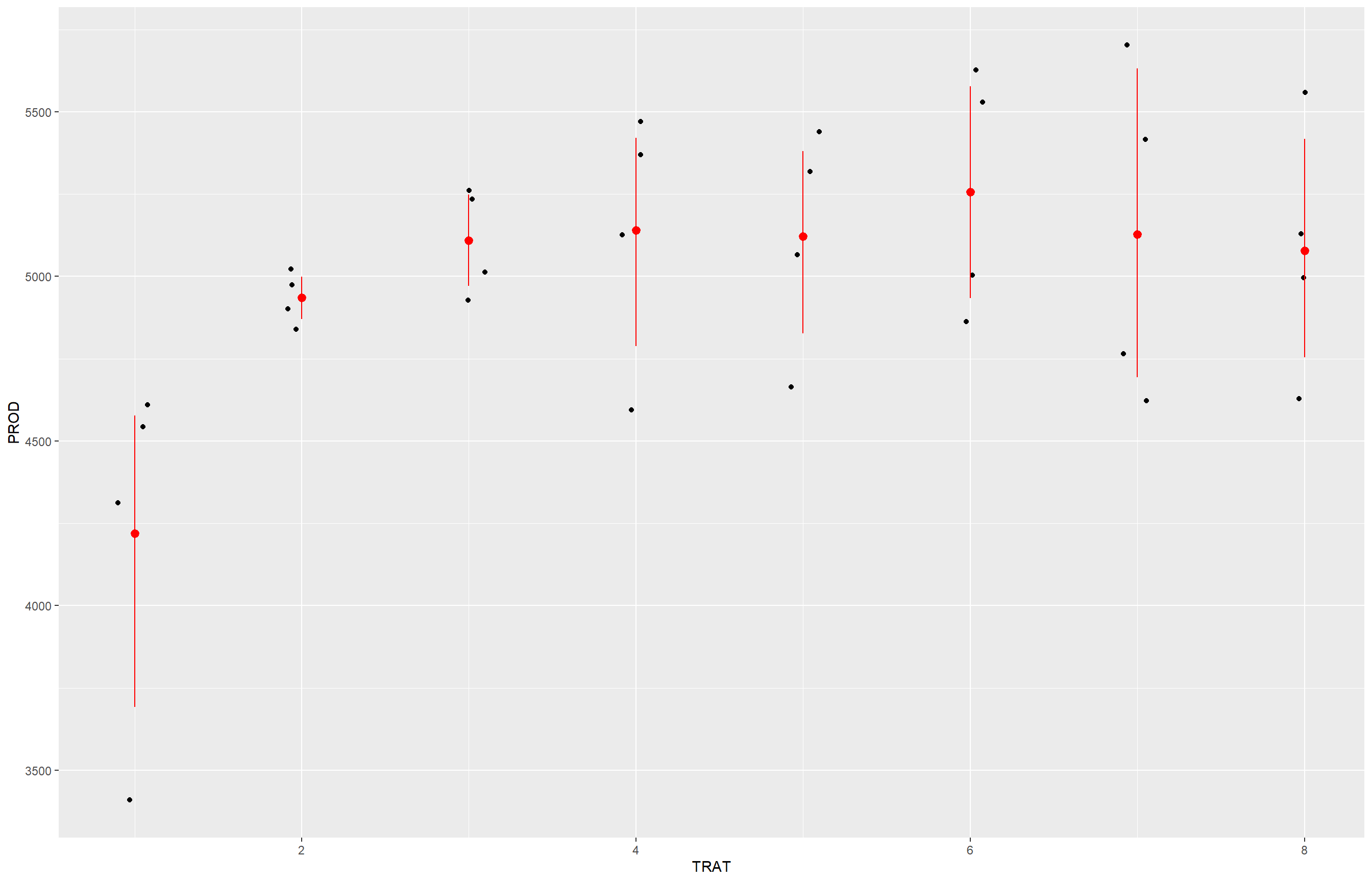

campo$TRAT <- factor (campo$TRAT)
campo$BLOCO <- factor (campo$BLOCO)

m_campo <- lm(PROD ~ BLOCO + TRAT, data = campo)
m_campo


Call:
lm(formula = PROD ~ BLOCO + TRAT, data = campo)

Coefficients:
(Intercept)       BLOCO2       BLOCO3       BLOCO4        TRAT2        TRAT3  
     4312.1       -156.4        -99.5       -115.4        715.8        890.8  
      TRAT4        TRAT5        TRAT6        TRAT7        TRAT8  
      921.0        902.8       1037.0        908.3        859.0

anova(m_campo)

Analysis of Variance Table

Response: PROD
          Df  Sum Sq Mean Sq F value  Pr(>F)  
BLOCO      3  105665   35222  0.2171 0.88340  
TRAT       7 2993906  427701  2.6367 0.04021 *
Residuals 21 3406431  162211                  
---
Signif. codes:  0 '***' 0.001 '**' 0.01 '*' 0.05 '.' 0.1 ' ' 1

means_campo <- emmeans(m_campo, ~ TRAT)
means_campo

 TRAT emmean  SE df lower.CL upper.CL
 1      4219 201 21     3800     4638
 2      4935 201 21     4516     5354
 3      5110 201 21     4691     5529
 4      5140 201 21     4721     5559
 5      5122 201 21     4703     5541
 6      5256 201 21     4837     5675
 7      5128 201 21     4709     5546
 8      5078 201 21     4659     5497

Results are averaged over the levels of: BLOCO 
Confidence level used: 0.95

plot(means_campo)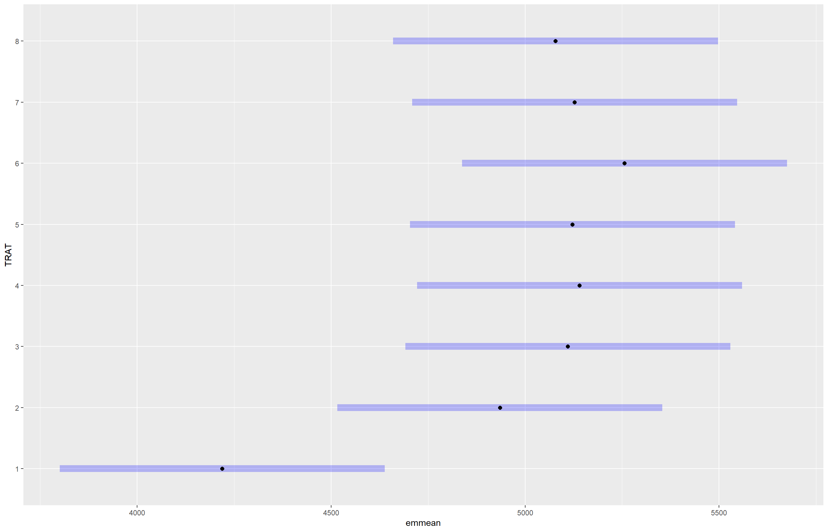

library(multcomp)
cld(means_campo)

 TRAT emmean  SE df lower.CL upper.CL .group
 1      4219 201 21     3800     4638  1    
 2      4935 201 21     4516     5354  12   
 8      5078 201 21     4659     5497  12   
 3      5110 201 21     4691     5529  12   
 5      5122 201 21     4703     5541  12   
 7      5128 201 21     4709     5546  12   
 4      5140 201 21     4721     5559  12   
 6      5256 201 21     4837     5675   2   

Results are averaged over the levels of: BLOCO 
Confidence level used: 0.95 
P value adjustment: tukey method for comparing a family of 8 estimates 
significance level used: alpha = 0.05 
NOTE: If two or more means share the same grouping symbol,
      then we cannot show them to be different.
      But we also did not show them to be the same.

m_campo <- lm(log(FER) ~ BLOCO + TRAT, data = campo)
m_campo


Call:
lm(formula = log(FER) ~ BLOCO + TRAT, data = campo)

Coefficients:
(Intercept)       BLOCO2       BLOCO3       BLOCO4        TRAT2        TRAT3  
     3.1347      -0.1964      -0.1878      -0.1675      -1.2600      -1.6600  
      TRAT4        TRAT5        TRAT6        TRAT7        TRAT8  
    -1.8718      -1.8211      -1.9052      -1.7825      -1.7491

anova(m_campo)

Analysis of Variance Table

Response: log(FER)
          Df  Sum Sq Mean Sq F value    Pr(>F)    
BLOCO      3  0.2064 0.06880  1.7961    0.1788    
TRAT       7 11.5210 1.64585 42.9665 4.838e-11 ***
Residuals 21  0.8044 0.03831                      
---
Signif. codes:  0 '***' 0.001 '**' 0.01 '*' 0.05 '.' 0.1 ' ' 1

library(DHARMa)
plot(simulateResiduals(m_campo))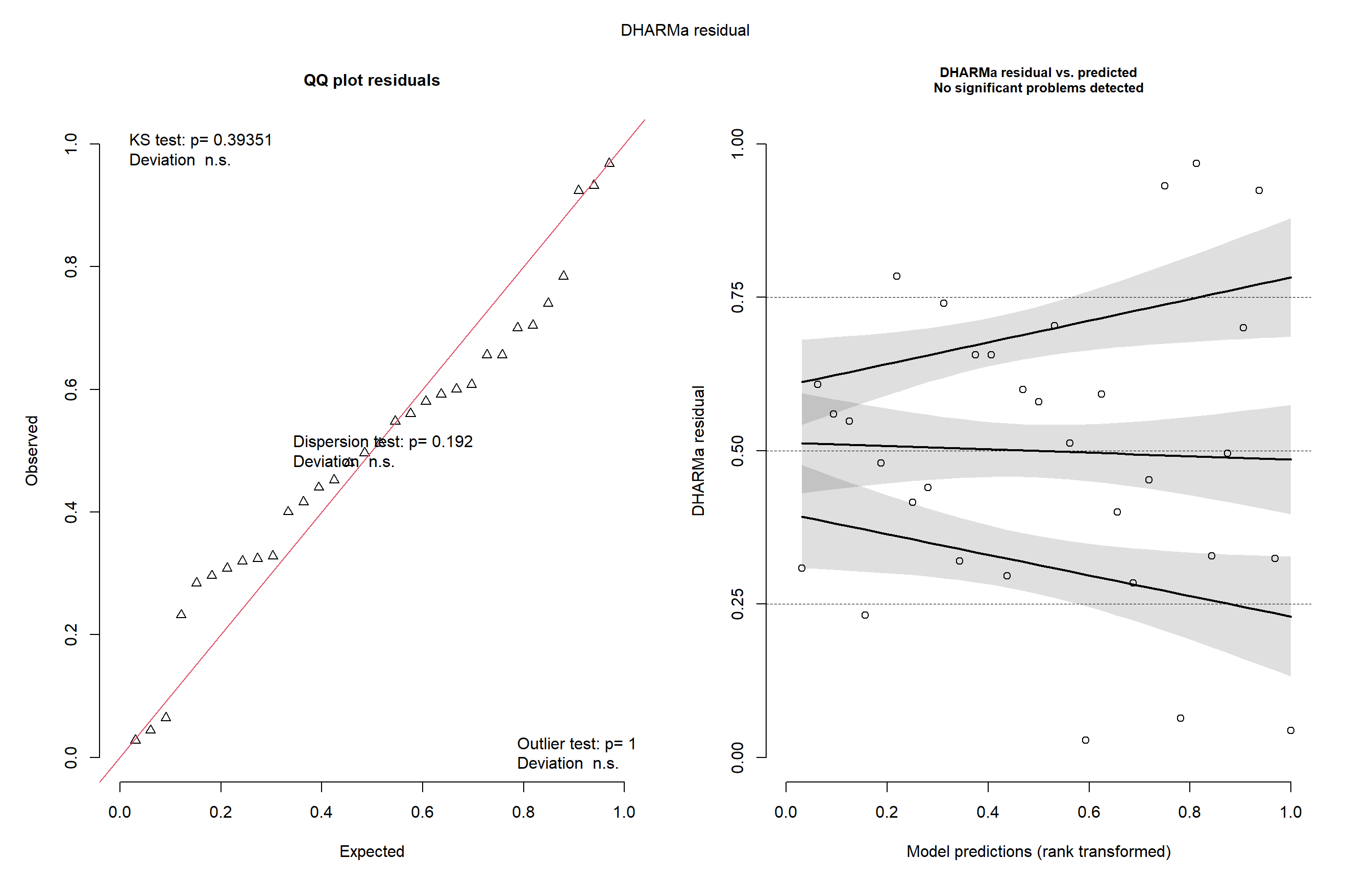

means_campo <- emmeans(m_campo, ~ TRAT, type = "response")
means_campo

 TRAT response    SE df lower.CL upper.CL
 1       20.02 1.960 21    16.33    24.54
 2        5.68 0.556 21     4.63     6.96
 3        3.81 0.373 21     3.11     4.67
 4        3.08 0.301 21     2.51     3.78
 5        3.24 0.317 21     2.64     3.97
 6        2.98 0.292 21     2.43     3.65
 7        3.37 0.330 21     2.75     4.13
 8        3.48 0.341 21     2.84     4.27

Results are averaged over the levels of: BLOCO 
Confidence level used: 0.95 
Intervals are back-transformed from the log scale

plot(means_campo)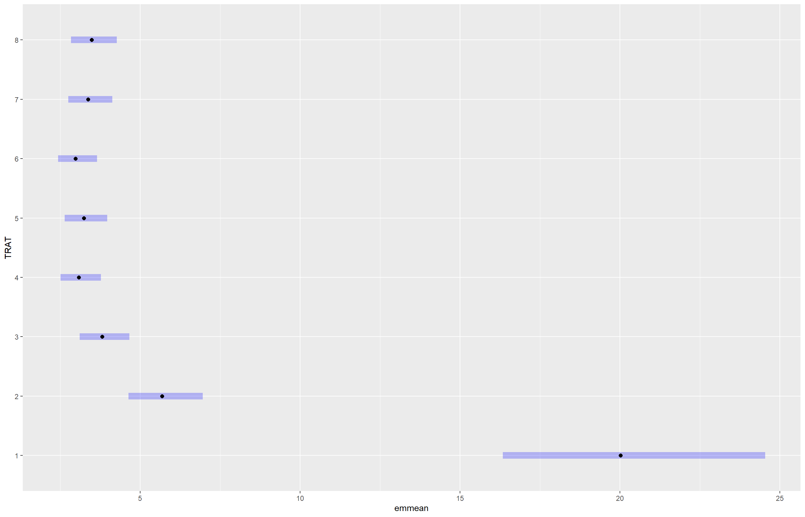

library(multcomp)
cld(means_campo)

 TRAT response    SE df lower.CL upper.CL .group
 6        2.98 0.292 21     2.43     3.65  1    
 4        3.08 0.301 21     2.51     3.78  1    
 5        3.24 0.317 21     2.64     3.97  1    
 7        3.37 0.330 21     2.75     4.13  1    
 8        3.48 0.341 21     2.84     4.27  1    
 3        3.81 0.373 21     3.11     4.67  12   
 2        5.68 0.556 21     4.63     6.96   2   
 1       20.02 1.960 21    16.33    24.54    3  

Results are averaged over the levels of: BLOCO 
Confidence level used: 0.95 
Intervals are back-transformed from the log scale 
P value adjustment: tukey method for comparing a family of 8 estimates 
Tests are performed on the log scale 
significance level used: alpha = 0.05 
NOTE: If two or more means share the same grouping symbol,
      then we cannot show them to be different.
      But we also did not show them to be the same.

pwpm(means_campo)

        1       2       3       4       5       6       7       8
1 [20.02]  <.0001  <.0001  <.0001  <.0001  <.0001  <.0001  <.0001
2   3.525 [ 5.68]  0.1252  0.0048  0.0110  0.0028  0.0204  0.0343
3   5.259   1.492 [ 3.81]  0.7832  0.9335  0.6440  0.9843  0.9976
4   6.500   1.844   1.236 [ 3.08]  0.9999  1.0000  0.9976  0.9842
5   6.178   1.753   1.175   0.951 [ 3.24]  0.9984  1.0000  0.9994
6   6.721   1.906   1.278   1.034   1.088 [ 2.98]  0.9842  0.9431
7   5.945   1.686   1.130   0.915   0.962   0.885 [ 3.37]  1.0000
8   5.750   1.631   1.093   0.885   0.931   0.856   0.967 [ 3.48]

Row and column labels: TRAT
Upper triangle: P values   null = 1  adjust = "tukey"
Diagonal: [Estimates] (response)   type = "response"
Lower triangle: Comparisons (ratio)   earlier vs. later

Aqui nós importamos os dados da planilha compartilhada pelo professor, depois visualizamos os dados usando um gráfico de dispersão com intervalos de confiança, o que mostra as diferenças de produtividade e entre os tratamentos. Convertemos as variáveis TRAT e BLOCO em fatores e, em seguida, ajustamos a ANOVA usando lm(PROD ~ BLOCO + TRAT) para avaliar o efeito dos tratamentos, considerando os blocos como fator de controle. Aplicamos a função anova() para verificar a significância das diferenças.

Utilizamos o pacote emmeans para estimar as médias ajustadas dos tratamentos e o cld() para realizar comparações múltiplas, identificando quais tratamentos diferem entre si estatisticamente. Depois avaliamos a variável FER, e ela não atendeu aos pressupostos do modelo, aplicamos uma transformação logarítmica. Ajustamos novamente o modelo e usamos o pacote DHARMa para verificar os resíduos simulados. E terminamos calculando as médias ajustadas transformadas de volta à escala original (type = “response”) e realizamos novas comparações com cld() e pwpm(), para verificar quais tratamentos apresentaram diferenças significativas em relação à fertilidade.

milho <- gsheet2tbl("https://docs.google.com/spreadsheets/d/1bq2N19DcZdtax2fQW9OHSGMR0X2__Z9T/edit?gid=1345524759#gid=1345524759")
view(milho)

milho |> 
  ggplot(aes(hybrid, index, color = method))+
  geom_jitter(width = 0.1)+
  coord_flip()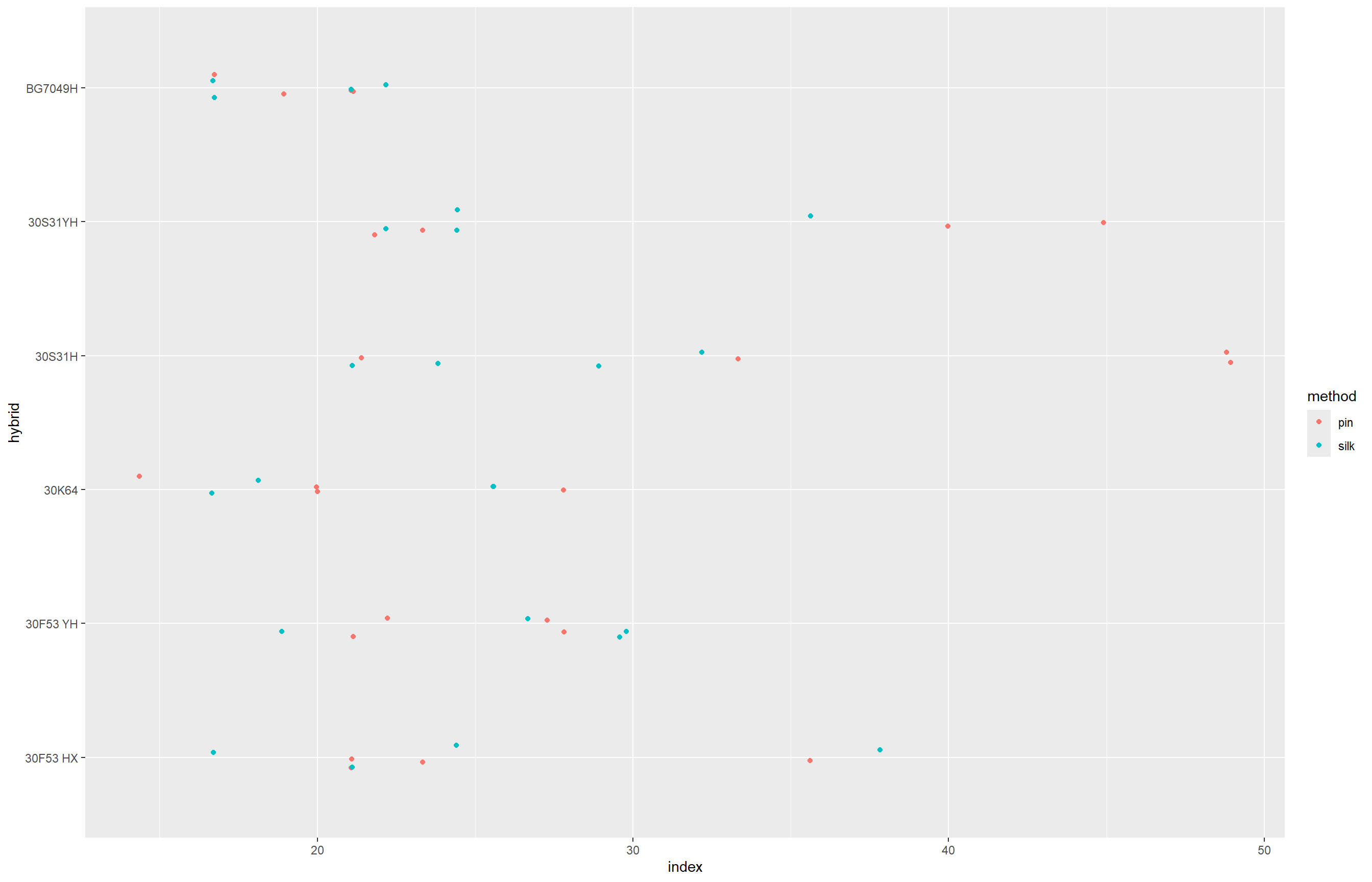

milho$hybrid_block <- interaction(milho$hybrid, milho$block)

library(dplyr)
milho |> 
  mutate(hybrid_block = interaction(hybrid, block))

# A tibble: 48 × 6
   hybrid   block method index yield hybrid_block
   <chr>    <dbl> <chr>  <dbl> <dbl> <fct>       
 1 30F53 HX     1 pin     21.1 12920 30F53 HX.1  
 2 30F53 HX     2 pin     21.1  9870 30F53 HX.2  
 3 30F53 HX     3 pin     23.3  8920 30F53 HX.3  
 4 30F53 HX     4 pin     35.6 13120 30F53 HX.4  
 5 30F53 YH     1 pin     21.1 12060 30F53 YH.1  
 6 30F53 YH     2 pin     22.2  7860 30F53 YH.2  
 7 30F53 YH     3 pin     27.3  7410 30F53 YH.3  
 8 30F53 YH     4 pin     27.8 10300 30F53 YH.4  
 9 30K64        1 pin     20   11700 30K64.1     
10 30K64        2 pin     20   10700 30K64.2     
# ℹ 38 more rows

library(DHARMa)
library(lme4)
m_milho <- lmer(index ~ hybrid*method + 
                  (1 | block:hybrid_block),
                data = milho)
car::Anova(m_milho)

Analysis of Deviance Table (Type II Wald chisquare tests)

Response: index
                Chisq Df Pr(>Chisq)   
hybrid        11.4239  5    0.04359 * 
method         4.6964  1    0.03023 * 
hybrid:method 15.8062  5    0.00742 **
---
Signif. codes:  0 '***' 0.001 '**' 0.01 '*' 0.05 '.' 0.1 ' ' 1

plot(simulateResiduals(m_milho))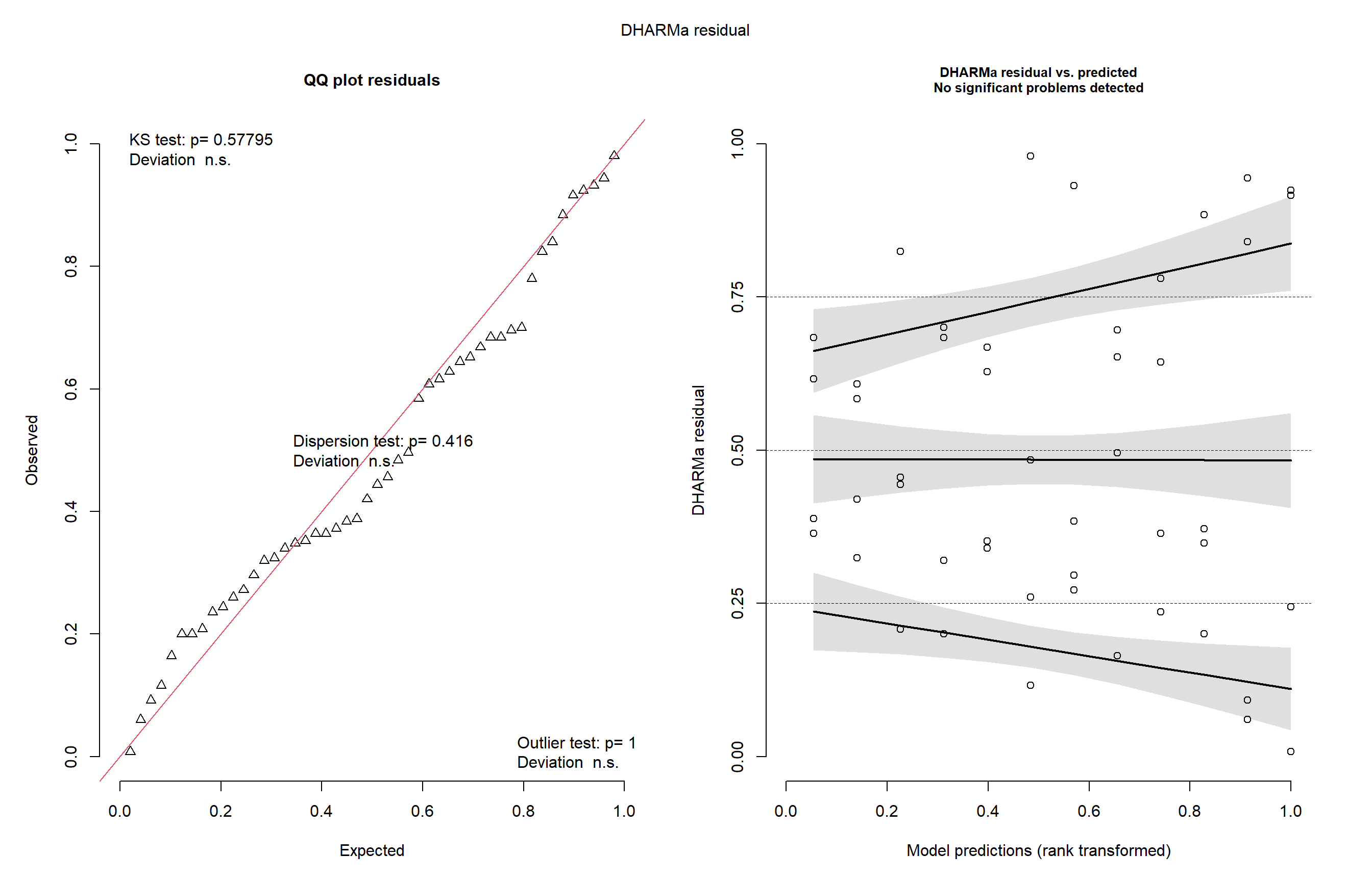

library(multcomp)
media_milho <- emmeans(m_milho, ~ hybrid | method)
cld (media_milho, Letters = letters)

method = pin:
 hybrid   emmean   SE   df lower.CL upper.CL .group
 BG7049H    19.4 3.57 24.9     12.1     26.8  a    
 30K64      20.6 3.57 24.9     13.2     27.9  a    
 30F53 YH   24.6 3.57 24.9     17.3     31.9  ab   
 30F53 HX   25.3 3.57 24.9     17.9     32.6  ab   
 30S31YH    32.5 3.57 24.9     25.2     39.8  ab   
 30S31H     38.1 3.57 24.9     30.8     45.4   b   

method = silk:
 hybrid   emmean   SE   df lower.CL upper.CL .group
 BG7049H    19.2 3.57 24.9     11.8     26.5  a    
 30K64      21.5 3.57 24.9     14.2     28.8  a    
 30F53 HX   25.0 3.57 24.9     17.7     32.3  a    
 30F53 YH   26.2 3.57 24.9     18.9     33.6  a    
 30S31H     26.5 3.57 24.9     19.2     33.8  a    
 30S31YH    26.6 3.57 24.9     19.3     34.0  a    

Degrees-of-freedom method: kenward-roger 
Confidence level used: 0.95 
P value adjustment: tukey method for comparing a family of 6 estimates 
significance level used: alpha = 0.05 
NOTE: If two or more means share the same grouping symbol,
      then we cannot show them to be different.
      But we also did not show them to be the same.

m_milho3 <- lmer(yield ~ hybrid*method + 
                  (1 | block:hybrid_block),
                data = milho)
car::Anova(m_milho3)

Analysis of Deviance Table (Type II Wald chisquare tests)

Response: yield
                Chisq Df Pr(>Chisq)    
hybrid        22.5966  5  0.0004031 ***
method         0.1052  1  0.7456932    
hybrid:method 25.9302  5  9.206e-05 ***
---
Signif. codes:  0 '***' 0.001 '**' 0.01 '*' 0.05 '.' 0.1 ' ' 1

plot(simulateResiduals(m_milho3))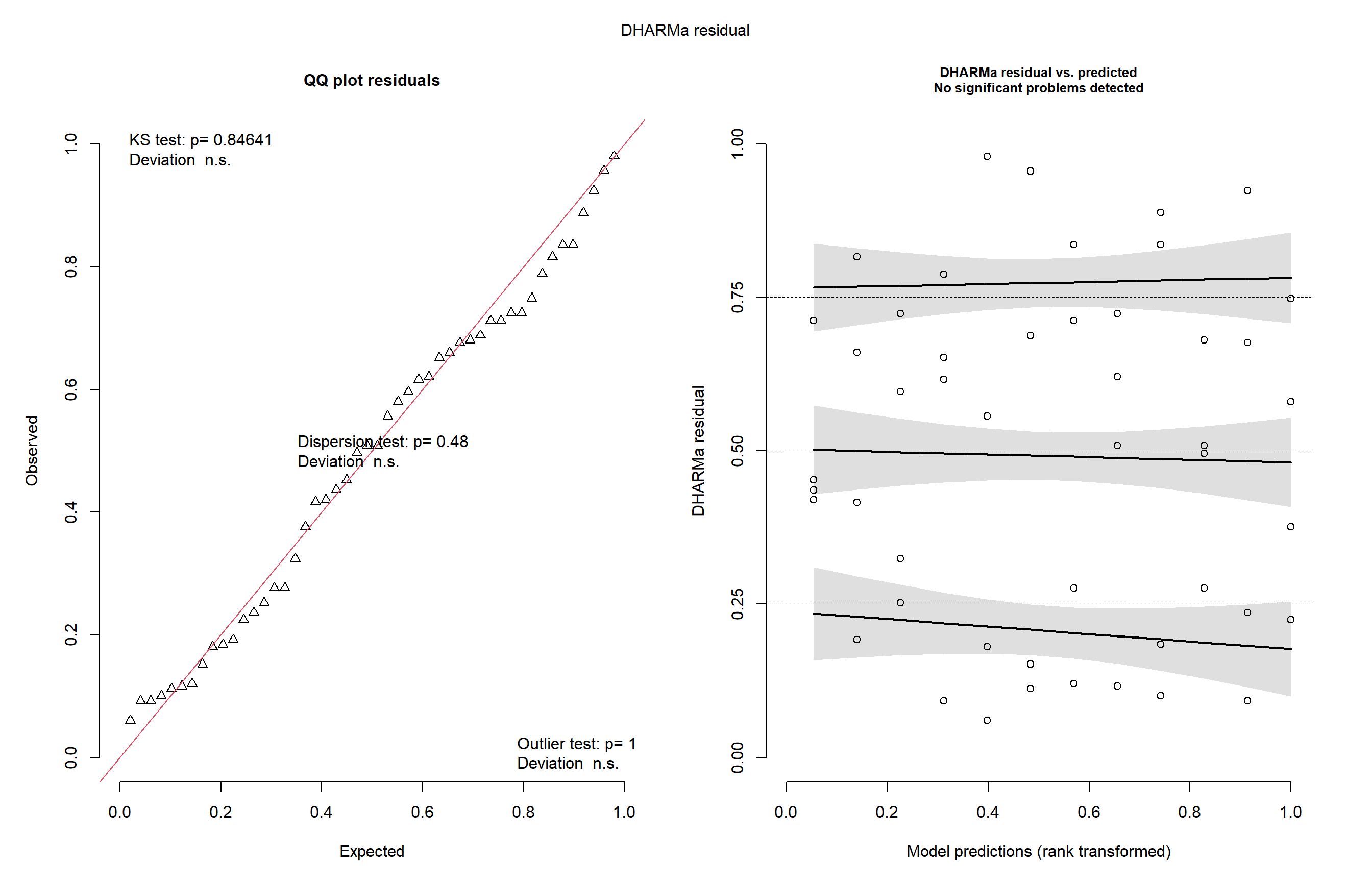

Aqui Importamos os dados do experimento com milho e visualizamos a variável index por híbrido e método. Criamos a variável hybrid_block para representar a interação entre híbrido e bloco, usada na modelagem mista com lmer(), considerando index como resposta e block:hybrid_block como efeito aleatório. Avaliamos os resíduos simulados com o pacote DHARMa e, com emmeans, estimamos as médias ajustadas dos híbridos por método, comparando-as com cld(). Repetimos o processo para a variável yield, ajustando novo modelo misto e verificando a qualidade do ajuste da mesma forma.

library(ggplot2)
milho |> 
  ggplot(aes(index,  yield))+
  geom_point()+
  geom_smooth(method = "lm")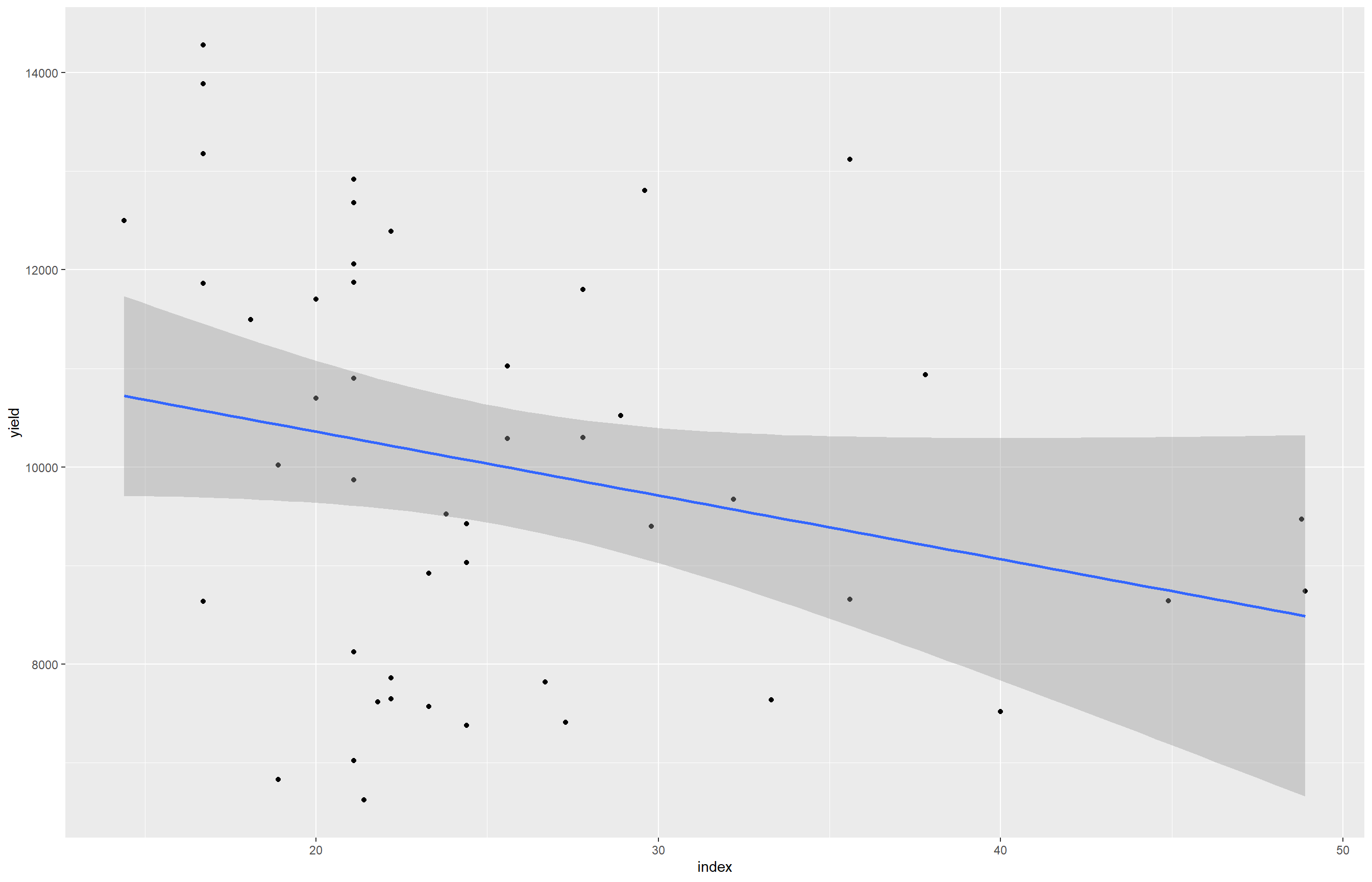

cor1 <- cor.test(milho$index, milho$yield)
R2_percentual <- (cor1$estimate)^2 * 100
R2_percentual*100

     cor 
632.3713

Aqui criamos um gráfico de dispersão com linha de tendência linear entre index e yield. Em seguida, calculamos a correlação entre as duas variáveis e obtivemos o R² percentual, que indica o quanto index explica a variação em yield.