Mapa e Site

Apresentação do site

O conjunto de dados será o da ferrugem do café na Etiópia que está no arquivo de dados na nuvem.

Utilizamos função gsheet2tbl() do pacote [gsheet] para carregar os dados no ambiente

library(gsheet)
cr <- gsheet2tbl("https://docs.google.com/spreadsheets/d/1bq2N19DcZdtax2fQW9OHSGMR0X2__Z9T/edit?gid=1871397229#gid=1871397229")
cr

# A tibble: 405 × 13
    farm region zone       district      lon   lat altitude cultivar shade    
   <dbl> <chr>  <chr>      <chr>       <dbl> <dbl>    <dbl> <chr>    <chr>    
 1     1 SNNPR  Bench Maji Debub Bench  35.4  6.90     1100 Local    Sun      
 2     2 SNNPR  Bench Maji Debub Bench  35.4  6.90     1342 Mixture  Mid shade
 3     3 SNNPR  Bench Maji Debub Bench  35.4  6.90     1434 Mixture  Mid shade
 4     4 SNNPR  Bench Maji Debub Bench  35.4  6.90     1100 Local    Sun      
 5     5 SNNPR  Bench Maji Debub Bench  35.4  6.90     1400 Local    Sun      
 6     6 SNNPR  Bench Maji Debub Bench  35.4  6.90     1342 Mixture  Mid shade
 7     7 SNNPR  Bench Maji Debub Bench  35.4  6.90     1432 Mixture  Mid shade
 8     8 SNNPR  Bench Maji Debub Bench  35.4  6.90     1100 Local    Sun      
 9     9 SNNPR  Bench Maji Debub Bench  35.4  6.89     1400 Local    Sun      
10    10 SNNPR  Bench Maji Debub Bench  35.4  6.88     1342 Mixture  Mid shade
# ℹ 395 more rows
# ℹ 4 more variables: cropping_system <chr>, farm_management <chr>, inc <dbl>,
#   sev2 <dbl>

library(DT)
datatable(cr)

library(tidyverse)
cr |> 
  ggplot(aes(lon, lat))+
  geom_point()

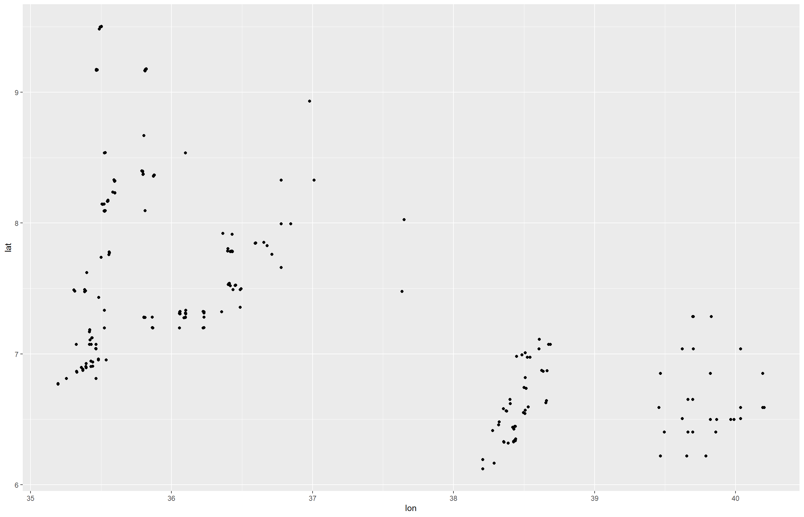
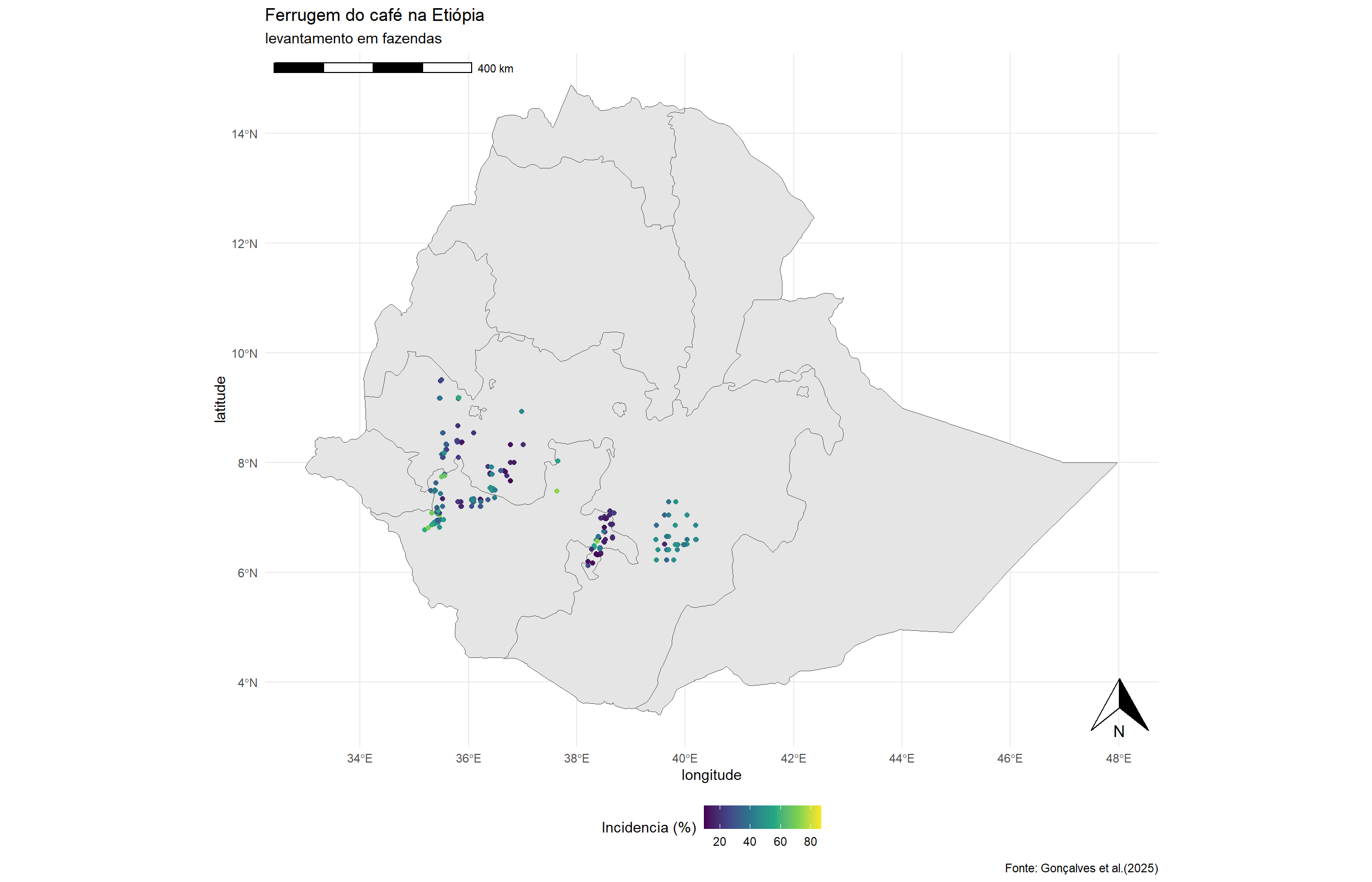
remotes::install_github("ropensci/rnaturalearthhires")
remotes::install_github("ropensci/rnaturalearth")


library(rnaturalearth)
library(sf)
library(earth)
ETH <- ne_states(country = "Ethiopia", 
                 returnclass = "sf")

library(tidyverse)
library(ggthemes)
library(ggspatial)

ggplot(ETH)+
  geom_sf(fill = "gray90")+
  geom_point(data = cr, aes(lon, lat, color = inc))+
  scale_color_viridis_c()+
  theme_minimal()+
  theme(legend.position = "bottom")+
  annotation_scale(location = "tl")+
  annotation_north_arrow(location = "br", which_north = "true")+
  labs(title = "Ferrugem do café na Etiópia", x = "longitude", y= "latitude", subtitle = "levantamento em fazendas", caption = "Fonte: Gonçalves et al.(2025)", 
       color = "Incidencia (%)")

ggsave("mapa.Etiópia.png", bg = "white", width = 10)

Aqui visualizamos os pontos em um gráfico simples, depois carregamos os limites geográficos do país usando o pacote rnaturalearth com o sf. Criamos um mapa temático com o ggplot2, mostrando a localização das fazendas coloridas conforme a incidência da doença. Adicionamos escala e seta de norte, aplicamos um tema limpo e salvamos o mapa em alta qualidade como imagem PNG.